Demand Forecasting with Amazon BSR & Sales Data Guide

In the competitive Amazon marketplace, staying ahead requires more than just a great product; it demands a data-driven strategy. Two of the most critical components of this strategy are demand forecasting and inventory optimization. Misjudge demand, and you risk costly overstocking or missed sales from stockouts. This guide will walk you through how to leverage Amazon's Best Sellers Rank (BSR) and historical sales data to create accurate demand forecasts and optimize your inventory levels, ensuring you have the right products in the right quantities at the right time.

What is Amazon Best Sellers Rank (BSR) and Why Does It Matter?

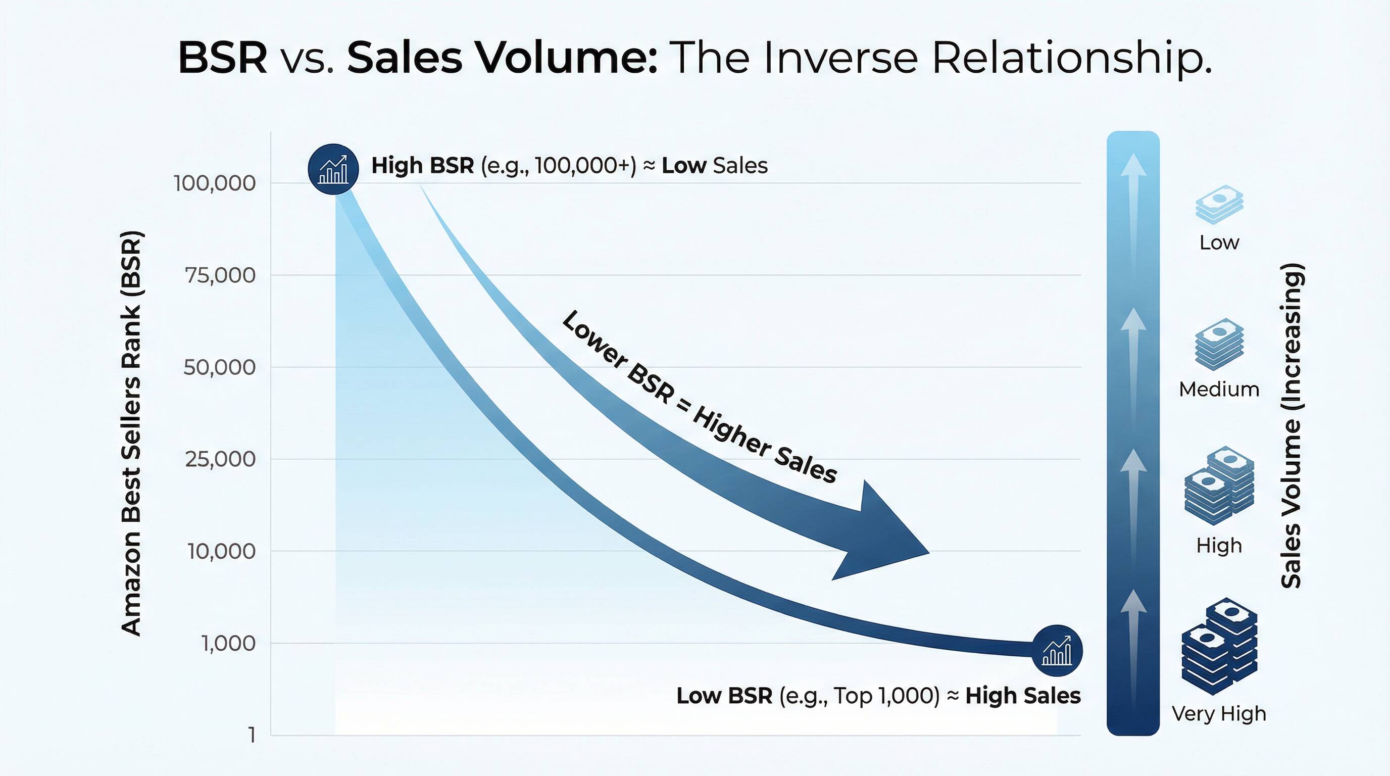
Amazon's Best Sellers Rank (BSR) is a powerful, near real-time indicator of a product's sales velocity within a specific category. A lower BSR means higher sales. For example, a product with a BSR of #10 is selling significantly more units than a product with a BSR of #10,000 in the same category. Because BSR is updated hourly, it provides a dynamic view of a product's performance, making it an invaluable metric for demand forecasting.

By tracking BSR over time, you can identify trends, seasonality, and the impact of marketing campaigns or pricing changes. This historical BSR data, when combined with other metrics, allows you to move beyond simple guesswork and create sophisticated models to predict future sales with a higher degree of accuracy.

The Power of Historical Sales Data

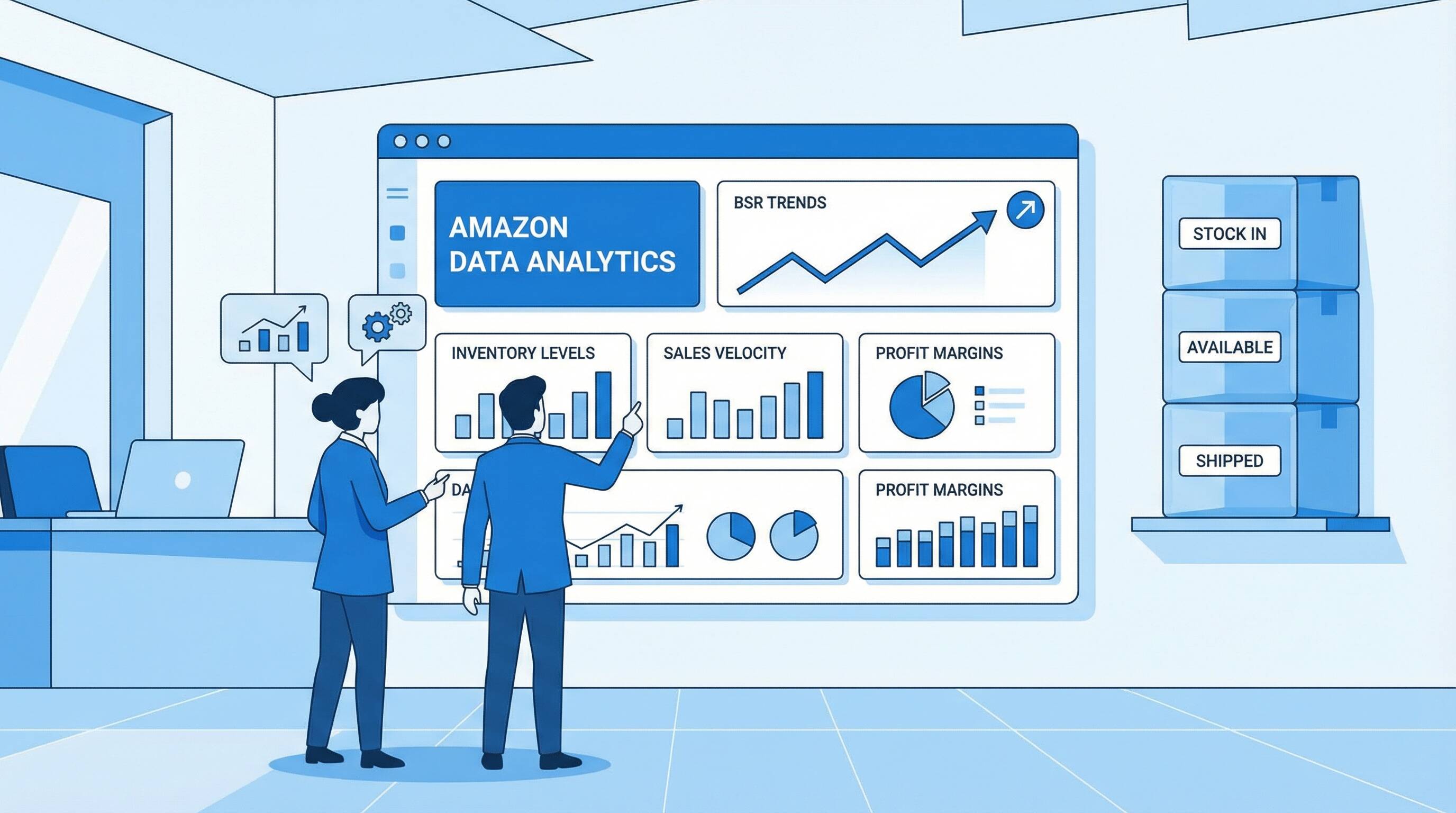
While BSR provides a relative measure of performance, historical sales data gives you the absolute numbers needed for precise forecasting. Analyzing past sales data allows you to:

• Identify Sales Velocity: Understand how many units of a product are sold per day, week, or month.
• Recognize Seasonality: Pinpoint predictable peaks and troughs in demand, such as holiday rushes or seasonal lulls.
• Measure Growth Trends: Determine if a product's sales are growing, declining, or plateauing over time.
• Analyze Price Elasticity: See how changes in price have historically affected sales volume.

By combining these insights, you can build a robust baseline for your demand forecast. For example, if you know a product's sales typically increase by 50% in December, you can proactively adjust your inventory to meet that demand.

How to Collect BSR and Sales Data with Easyparser

Manually tracking BSR and sales data is time-consuming and prone to errors. Easyparser automates this process, allowing you to collect accurate, real-time, and historical data at scale. Here’s how you can use Easyparser's API to gather the data you need for demand forecasting:

Using the Sales Analysis & History Operation

The SALES_ANALYSIS_HISTORY operation is your all-in-one tool for deep product intelligence. With a single request, you can retrieve up to 12 months of historical data, including weekly trends in BSR, sales, pricing, and more. This is the data that will form the backbone of your demand forecast.

For a comprehensive overview of this operation's capabilities, including traffic intelligence, profitability metrics, and use cases, visit the Sales Analysis & History Documentation.

Here is a Python example of how to use the Easyparser API to get sales analysis and history for a specific product. For detailed information about all available request parameters and their usage, check out the Request Documentation.

import requests
import json
params = {
'api_key': 'YOUR_API_KEY',
'platform': 'AMZ',
'operation': 'SALES_ANALYSIS_HISTORY',
'domain': '.com',
'asin': 'B08BHSYQ9C',
'history_range': '12'
}
api_result = requests.get('https://realtime.easyparser.com/v1/request', params)
data = api_result.json()
# Extract historical data
historical_data = data.get('history', [])
for week in historical_data:
print(f"Week: {week['date']}, BSR: {week['bsr']}, Sales: {week['sales']}")

Example API Response

When you call the API with the above parameters, you'll receive a comprehensive JSON response containing detailed product information and historical data. Here's a sample response for the example ASIN:

{
"result": {
"product": {
"asin": "B08BHSYQ9C",
"name": "Brizled Color Changing Halloween Lights...",
"brand": "Brizled",
"category": "Seasonal Décor/Seasonal Lighting/Indoor String Lights",
"currency": "USD",
"age": 5.4,
"performance": {
"traffic": {
"views_last_30_days": 37616,
"views_last_90_days": 59334,
"month_over_month_change": 1.64
},
"sales": {
"purchases_last_30_days": 3003,
"purchases_last_90_days": 4737,
"purchases_last_360_days": 6182
}
},
"pricing": {
"average_price_last_90_days": 28.30,
"average_price_last_360_days": 30.06
},
"reviews_and_ranking": {
"reviews": {
"total_count": 7047,
"average_rating": 4.1
},
"ranking": {
"current_rank": 18,
"category": "Indoor String Lights",
"average_rank": 33.92
}
}
},
"history": [
{
"date": "2025-12-07T00:00:00.000Z",
"views": 11985,
"purchases": 956,
"average_price": 24.73,
"best_seller_rank": 38
},
{
"date": "2025-11-30T00:00:00.000Z",
"views": 6768,
"purchases": 540,
"average_price": 25.38,
"best_seller_rank": 44
},
{
"date": "2025-11-23T00:00:00.000Z",
"views": 3647,
"purchases": 291,
"average_price": 25.51,
"best_seller_rank": 51
}
// ... more historical data
]
}
}

This response provides everything you need for demand forecasting: current performance metrics, pricing trends, and weekly historical data showing how views, purchases, price, and BSR have changed over time. You can use this data to identify patterns, calculate sales velocity, and build accurate forecasts.

To understand every field in the response and how to leverage the data effectively, refer to the complete Response Documentation.

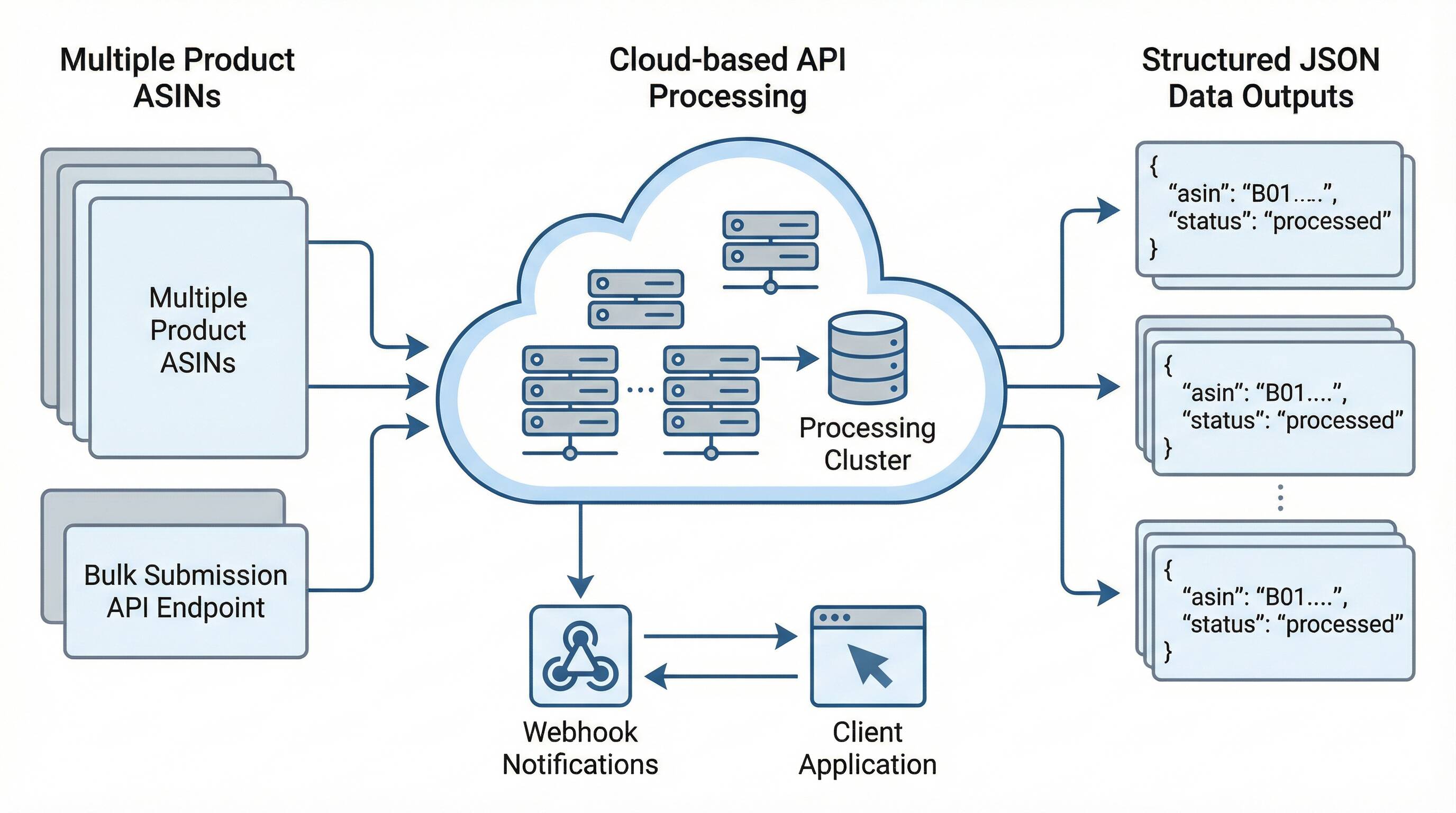
Using the Bulk API for Large-Scale Analysis

For serious sellers managing hundreds or thousands of products, the Bulk API is a game-changer. You can submit a list of ASINs and retrieve historical data for all of them asynchronously. This allows you to build a comprehensive view of your entire product catalog and make data-driven decisions at scale.

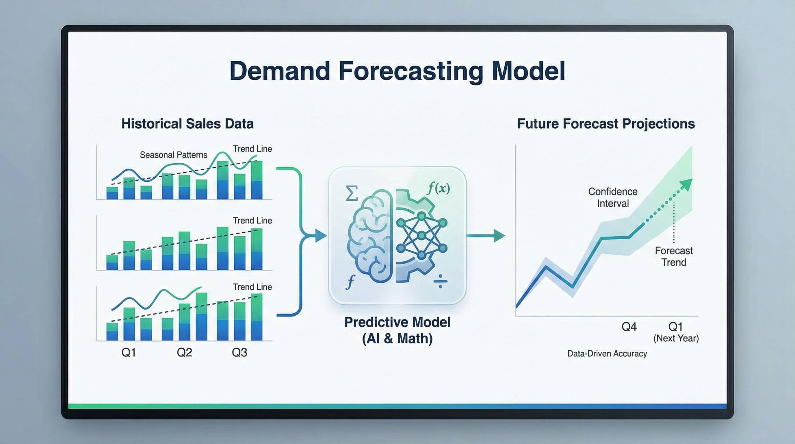
Strategies for Demand Forecasting with BSR and Sales Data

Once you have collected your data, you can start building your demand forecast. Here are a few strategies you can use:

1. Time Series Analysis

Time series analysis involves analyzing your historical sales data to identify patterns and trends. You can use techniques like moving averages to smooth out short-term fluctuations and identify the long-term trend. For example, a 4-week moving average can help you see the underlying sales trend without being distracted by weekly noise.

2. Seasonal Decomposition

If your products have strong seasonality, you can use seasonal decomposition to separate the underlying trend from the seasonal effects. This will allow you to forecast the baseline demand and then add the seasonal component back in to get your final forecast.

3. Predictive Modeling

For more advanced forecasting, you can use predictive modeling techniques like regression analysis. You can build a model that uses BSR, price, and other factors to predict future sales. This can be particularly useful for understanding the relationship between different variables and how they impact sales.

From Forecasting to Inventory Optimization

An accurate demand forecast is the foundation of effective inventory management. Once you know how much you are likely to sell, you can make informed decisions about how much inventory to hold. Here are some key inventory optimization techniques:

1. Calculating Safety Stock

Safety stock is the extra inventory you hold to protect against unexpected surges in demand or delays in your supply chain. A good starting point is to calculate your average daily sales and your supplier lead time. You can then use this formula to determine your safety stock:

(Maximum Daily Sales x Maximum Lead Time) - (Average Daily Sales x Average Lead Time)

You can use the historical sales data from Easyparser to calculate your average and maximum daily sales with a high degree of accuracy.

2. Determining Your Reorder Point

Your reorder point is the inventory level at which you need to place a new order to avoid a stockout. You can calculate your reorder point with this formula:

(Average Daily Sales x Lead Time) + Safety Stock

By setting a reorder point, you can automate your inventory management and ensure that you always have enough stock to meet demand.

3. Maintaining Optimal Inventory Levels

The goal of inventory optimization is to balance the cost of holding inventory with the risk of stockouts. A common rule of thumb for Amazon FBA sellers is to maintain 30-60 days of supply. By using your demand forecast, you can adjust your inventory levels to match the expected sales velocity, ensuring you don't tie up too much capital in slow-moving stock.

Conclusion: Turning Data into Profit

Demand forecasting and inventory optimization are not just theoretical exercises; they are essential practices for any successful Amazon business. By leveraging the power of Amazon BSR and historical sales data, you can move from reactive to proactive management, making data-driven decisions that boost profitability and drive growth. With a tool like Easyparser, you can automate the data collection process and focus on what really matters: building a thriving e-commerce business.